Finding the n most common entries in a list (Part 1)

I came across a problem a short while ago of how to determine the top 5 most common numbers (though in fact the data could be anything) in a range. Excel handily provides the “MODE()” function for determining the most common entry, but no more than that. Newer versions of Excel feature the “MODE.MULT” function, but this only returns multiple values that share the top spot, not the successors. Unfortunately, you can’t use the syntax of MODE(<range>,n) as you can for say LARGE()

I wanted to share this one as it provides a good example of the general process used to build a complex array formula.

The exact method for this process had eluded me for some time – I was able to come up with a basic version within a few minutes, but working round a major flaw took some thinking.

Here’s some example data we’re going to work from:

I’ve chosen the exact order of the numbers above to trigger some of the “gotcha”s that caused me the difficulty. The first column contains the 28 data points we’re analysing. The 2nd column is the result of the FREQUENCY function entered as an array running the input range as both the input and the bins (=FREQUENCY(A2:A29,A2:A29).)
This returns an array of the count of each entry on and only on the first time any particular value crops up. Any subsequent values return a zero. As an aside, this is the behaviour exploited for the original ‘count unique’ formula mentioned in an earlier post.

So far so good. Onto building the formula.

The way I, and many others go about working out a complex array formula is to break it into the constituent parts, and then piece them all together at the end bit by bit. Take a look at the Frequency column in the data above; you’ll see that in this data set, there are 6 twos, 4 threes, 2 fours, 1 five, 7 nines and 6 sixes. A total of 6 discrete original data values, and we want to know the top 5. A cursory glance over this small data set tells you that this is all of them apart from that single five. Five is indeed the loneliest num…. never mind.

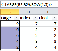
So for the next stage of the build, we want to know the 5 highest frequency entries. We run a LARGE function over the frequency values to find these.

=LARGE(B2:B29,ROW(1:5))

To see what the ROW function is doing here, check out the previous blog entry.

This shows us as the array result of a formula that the 5 highest frequencies are the nine, a couple of sixes, a four and a two, which agrees with the cursory glance from before. Perfect.

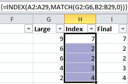
The next step here is to use these results and then perform a lookup to find out the original data values that caused them. A nested INDEX/MATCH combination does the job nicely:

=INDEX(A2:A29,MATCH(G2:G6,B2:B29,0))

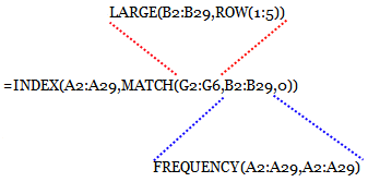
The final stage is to conglomerate all the helper columns into one final formula so that it refers only to the original data. Working right to left from the helper columns, replace anything referencing one of the helper build columns (B, G and H in this example) to the equivalent to its left.
So here, the INDEX/MATCH combination has two references that aren’t the original data in Column A, G2:G6 and B2:B29. Replace these with the formula from these ranges.

G2:G6 refers to our LARGE formula: =LARGE(B2:B29,ROW(1:5))
and B2:B29 refers to the FREQUENCY formula: =FREQUENCY(A2:A29,A2:A29)

These substitutions result in a formula of:
=INDEX(A2:A29,MATCH(LARGE(B2:B29,ROW(1:5)),FREQUENCY(A2:A29,A2:A29),0))

This substitution has resulted in one other reference to a helper column, B2:B29. Run through and replace this with its respective formula:
=INDEX(A2:A29,MATCH(LARGE(FREQUENCY(A2:A29,A2:A29),ROW(1:5)),FREQUENCY(A2:A29,A2:A29),0))

And there we have it, the process of building a complex array formula! The secrets are:

1. Use helper columns to get you to a place where you’ve got the intended result
2. Working backwards (right to left) across the helper columns, substitute in relevant sub-formula until you are only referencing the original data

Eagle eyed viewers may have noticed that this formula doesn’t quite give the final result we’re after. Where there are two values with the same frequency, the MATCH function picks up the first found original value for both (2 in this case). Stay tuned for the next post where I’ll talk about how to get round this limitation.